Popularity-bias Deconfounding (PD) - Estimation

Estimation method

Last time, we have identified the followiing causal effect. $$ \mathbb{E}\left[ C(i)\middle| U=u \right]=\mathbb{E}\left\{\mathbb{E}\left[ C\middle|I=i,U=u,Z \right]\right\}. $$

To estimate the statistical estimand on the RHS, we first estimate $\mathbb{E}\left[ C\middle|I=i,U=u,Z \right]$. This can be down with some traditional recommendation training method. For example, optimizing the pairwise BPR objective function on historical data $\mathcal{D}$: $$ \begin{aligned} \max_\Theta \sum_{(u,i,j)\in\mathcal{D}} \log \sigma ( \mathbb{E}_\Theta \left[ C\middle|I=i,U=u,Z=m_i^t \right] \\ - \mathbb{E}_\Theta \left[ C\middle|I=i,U=u,Z=m_j^t \right] ) - \lambda\left\Vert \Theta \right\Vert_2^2, \end{aligned} $$ where $\Theta$ denotes the parameters modeling $\mathbb{E}\left[ C\middle|I=i,U=u,Z \right]$, $j$ denotes the negative sample for $u$, $\sigma (\cdot)$ is the sigmoid function.

It remains to show how to parameterize $\mathbb{E}_\Theta \left[ C\middle|I=i,U=u,Z=m_i^t \right]$ specifically. To decouple the user-item match with item popularity, we design the model as: $$ \mathbb{E}_\Theta \left[ C\middle|I=i,U=u,Z=m_i^t \right] = ELU'(f_\Theta (u,i))\times (m_i^t)^\gamma, $$ where $f_\Theta (u,i)$ can be any user-item mathcing model and we choose the simple Matrix Factorization (MF) here; hyperparameter $\gamma$ is to control the strenth of conformity effect. $ELU’(\cdot)$ is a variant of the Exponential Unit active function that ensures the positivity of the matching score: $$ \begin{equation*} ELU'(x)= \begin{cases} e^x & \text{if } x \leq 0\\ x+1 & \text{else }. \end{cases} \end{equation*} $$

Lastly, since we are only interested in the rank of items, we do not need to normalize the estimation to make it a rigorous probability.

Now we move forward to estimate $\mathbb{E}\left\{\mathbb{E}\left[ C\middle|I=i,U=u,Z \right]\right\}$. Plug in the model for $\mathbb{E}_\Theta \left[ C\middle|I=i,U=u,Z \right]$.

$$ \begin{align} \mathbb{E}\left\{\mathbb{E}\left[ C\middle|I=i,U=u,Z \right]\right\} & = \mathbb{E}\left\{\mathbb{E}_\Theta \left[ C\middle|I=i,U=u,Z \right]\right\} \\ & = ELU'(f_\Theta (u,i))\times \mathbb{E}\left[Z^\gamma\right]. \end{align} $$

Notice that $ \mathbb{E}\left[Z^\gamma\right] $ is a constant. Ignoring it will not affect ranking. Hence, we can simply use $ ELU'(f_\Theta (u,i)) $ to estimate $\mathbb{E}\left[ C(i)\middle| U=u \right]$.

To summarize, we fit the historical interaction data with $\mathbb{E}_\Theta \left[ C\middle|I=i,U=u,Z=m_i^t \right]$, and use the user-item matching component $ ELU'(f_\Theta (u,i)) $ for deconfounded ranking. We name this method as Popularity-bias Deconfounding (PD). Combined with cross-validation, we have the following algorithm.

Datasets

In this article, experiments are conducted on three datasets. We summarize them in the following table.

dataset	output type	size
Kwai	clicking	7,658,510 interactions between 37,663 users and 128,879 items
Douban Movie	rating	7,174,218 interactions between 47,890 users and 26,047 items
Tencent	likes	1,816,046 interactions between 80,339 users and 27,070 items

From the table above, we can see that although we call $C$ “clicking”, it is not necessary to be 0-1 value. It can be integer-valued or continuously valued rating. This is why this blog use the notation $\mathbb{E}[C\ldots]$ instead of $\mathbb{P}(C=1\ldots)$ as in the orinal paper¹. As shown above, this method can be applied on large scale dataset. “Likes” are a little bit different from “clicking” since they are much more sparse. This is the reason why for the third dataset, we requires more interactions (we can manipulate the dataset by change the number of cores for filtering).

Performance

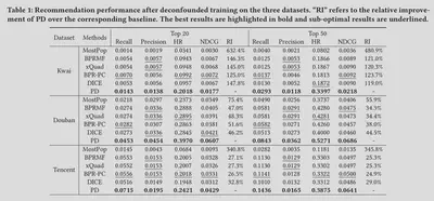
The proposed method (PD) are compared with a bunch of baseline methods, from heuristic methods like MostPop and MostRecent, to methods withour popularity adjustment such as BPRMF and state-of-art methods to handle popularity bias such as BPR-PC and DICE and so on. The propsed PD consistently outperforms all the baselines on all datasets. The degree of improvement depends on popularity properties of the datasets. Higher popularity drifts imply that item popularity $Z$ has larger impact on the recommendation data and PD achieves higher degree of improvement. The details are shown in the following table.

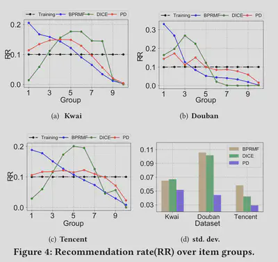
A recommendation analysis is conducted on some of these methods to show how much the recommendation favors popular items. In order to compare, they first design a metric called Recommendation Rate (RR). First, they sort the items in the recommendation list according to their popularity in descending order. Then, cut the sorted list into 10 pieces (groups) so that each group shares the same total popularity (the sum of popularity over all items). Now, we can define the RR of group $g$ as the ratio of the number of items comming from the group $g$ over the total number of recommended items. Formally, it can be define as

$$ RR(g,algo)=\frac{\sum_{i\in Group_g} RC(i,algo)}{\sum_{i\in Group_g} RC(i,algo)} $$ where $RC(i,algo)$ gives the number of times the algorithm $algo$ recommends item $i$ in the recommendation list.

As the figure above shows, although still going down, PD exhibits lines that are flatter than other methods, which means it performs better at eiliminating the effect of popularity when recommending items.

References

• [1] Causal Intervention for Leveraging Popularity Bias in Recommendation